Modified Mathieu as a Doubly Confluent Heun Realization

The symmetric quartic double well had polynomial tails and four sub-barrier turning points. Replace it by one real hyperbolic well and the boundary conditions remain two-sided decay, but the coordinate compactification changes completely: the two spatial ends become irregular singularities of a confluent Heun equation.

For the convention fixed below, the exact scalar statement is

$$\begin{gathered} H_\kappa=-\frac{\dd^2}{\dd x^2}+2\kappa\cosh(2x), \qquad H_\kappa\Phi=A\Phi, \qquad \Phi\in L^2(\mathbb R), \\ s=\ee^x, \qquad \zeta=-2\sqrt\kappa\,s, \qquad \Phi=s^{1/2}\ee^{-\sqrt\kappa(s+s^{-1})}Y(\zeta), \end{gathered}$$

where $Y$ obeys the DLMF doubly confluent Heun equation with

$$(\alpha_{\mathrm D},\gamma_{\mathrm D},\delta_{\mathrm D},q_{\mathrm D}) = \left(1,2,-4\kappa,2\kappa-A-\frac14\right).$$

The physical contour is the negative $\zeta$-ray. Decay selects the algebraic sectorial solution at each of its two irregular ends, so the spectrum is a connection-coefficient zero. The minimal ramified equation has Katz slopes $(1/2,1/2)$; consequently the associated pure isomonodromic system is P_{\mathrm{III}}(D_8)=P_{\mathrm{III}_3), even though its quadratic scalar lift has the standard rank-one/rank-one DCHE form.

First reading

Follow real-cosh passport → ramified equation → quadratic DCHE lift → endpoint branches → Wronskian zero → numerical table. The second-sheet gauge and tau-function checkpoint can wait for a second pass.

Status ledger

Statement	Status and scope
Operator properties, coordinate maps, gauges, and parameter dictionaries	Exact for $\kappa>0$
Endpoint formal series	Sectorial Poincaré asymptotics; truncation is not convergence
Abel-normalized Wronskian and parity conditions	Exact once the sectorial normalizations are fixed
Turning points	Exact for $A>2\kappa$ on the physical real sheet
Deep-well formula	Fixed-level asymptotic as $\kappa\to+\infty$
PIII(D₈) tau representation	Exact isomonodromic result in the cited monodromy chart, continued through resonant charts when necessary
Printed eigenvalues and residuals	Refined double-precision evidence, not certified intervals

A real-cosh passport fixes a discrete parity spectrum

Take $\kappa>0$ and let $H_\kappa$ be the Friedrichs realization of

$$-\frac{\dd^2}{\dd x^2}+2\kappa\cosh(2x)$$

on $L^2(\mathbb R)$. The potential is smooth, bounded below, and tends to $+\infty$ at both ends. Hence the resolvent is compact. One-dimensional Sturm–Liouville theory gives a simple ordered spectrum

$$2\kappa<A_0<A_1<A_2<\cdots,$$

and reflection symmetry makes the eigenfunctions alternate even, odd, even, odd, beginning with the positive even ground state. Equivalently, if $\Phi_R(x,A)$ is recessive as $x\to+\infty$, then

$$\begin{aligned} \Phi_R'(0,A_{2m})&=0, \\ \Phi_R(0,A_{2m+1})&=0. \end{aligned}$$

This is not the periodic problem of the Mathieu-band page. In the DLMF modified-Mathieu convention

$$w''-(a_{\mathrm M}-2q_{\mathrm M}\cosh 2x)w=0,$$

our confining slice is

$$(a_{\mathrm M},q_{\mathrm M})=(-A,-\kappa).$$

Thus a table written for positive $q_{\mathrm M}$ cannot be imported without analytic continuation and a new boundary-condition audit.

Two further dictionaries are useful. The mechanical pure-$SU(2)$ form

$$\left[ -\hbar_{\mathrm m}^2\frac{\dd^2}{\dd Q^2} +2\Lambda^2\cosh Q \right]\Psi=u\Psi$$

agrees after $Q=2x$ with

$$\kappa=\frac{4\Lambda^2}{\hbar_{\mathrm m}^2}, \qquad A=\frac{4u}{\hbar_{\mathrm m}^2}.$$

The $P_{\mathrm{III}}(D_8)$ normalization used later is

$$\left[ -\partial_Q^2+2\sqrt{t_{\mathrm{III}}}\cosh Q \right]\Psi=E_{\mathrm{III}}\Psi,$$

so that

$$t_{\mathrm{III}}=\frac{\kappa^2}{16}, \qquad E_{\mathrm{III}}=\frac A4.$$

These are convention maps, not additional quantization conditions.

The single exponential coordinate is still ramified

The economical coordinate for the two physical ends is

$$r=\ee^{2x}.$$

Since $\partial_x=2r\partial_r$, the eigenvalue equation becomes

$$\Phi_{rr}+\frac1r\Phi_r +\left( \frac{A}{4r^2} -\frac{\kappa}{4r} -\frac{\kappa}{4r^3} \right)\Phi=0.$$

Remove the first derivative by $\Phi=r^{-1/2}\chi$. At $r=0$ the normal form has a pole of order three, rather than the order-four pole of an unramified rank-one singularity. The same statement holds at infinity after inversion. Each endpoint therefore has Katz slope $1/2$.

The exact reduced form is especially transparent after

$$\xi=-\frac\kappa4r, \qquad q_{\mathrm{dr}}=-\frac{A+1}{4}, \qquad \epsilon_{\mathrm{dr}}=\frac{\kappa^2}{16}.$$

It is

$$\chi_{\xi\xi} +\frac{ \xi-q_{\mathrm{dr}}+\epsilon_{\mathrm{dr}}\xi^{-1} }{\xi^2}\chi=0.$$

This equation is called the doubly reduced doubly confluent Heun equation, or DRDCHE. Its square-root exponential characters at both ends display the $(1/2,1/2)$ formal type directly. The word “reduced” matters: this is not literally the four-parameter DLMF DCHE, and a software symbol named HeunD does not by itself denote either of its physical sectorial solutions.

A quadratic cover lands exactly in the DLMF DCHE

To unramify both ends, take the half-exponential coordinate

$$s=\ee^x, \qquad r=s^2, \qquad \zeta=-2\sqrt\kappa\,s.$$

The reduced and lifted coordinates satisfy

$$\xi=-\frac{\zeta^2}{16}.$$

Before any gauge transformation, the equation in $s$ is

$$\Phi_{ss}+\frac1s\Phi_s +\left( \frac A{s^2}-\kappa-\frac\kappa{s^4} \right)\Phi=0.$$

Now set $\rho=\sqrt\kappa>0$ and choose

$$\Phi=s^{1/2}\exp[-\rho(s+s^{-1})]Y(\zeta).$$

Direct differentiation first gives

$$\begin{aligned} Y_{ss} {}&+ \left( -2\rho+\frac2s+\frac{2\rho}{s^2} \right)Y_s \\ &+ \left[ -\frac{2\rho}{s} +\frac{A+1/4-2\kappa}{s^2} \right]Y=0. \end{aligned}$$

Using $\zeta=-2\rho s$ converts this exactly to

$$Y''+ \left( 1+\frac{\gamma_{\mathrm D}}{\zeta} +\frac{\delta_{\mathrm D}}{\zeta^2} \right)Y' +\left( \frac{\alpha_{\mathrm D}}{\zeta} -\frac{q_{\mathrm D}}{\zeta^2} \right)Y=0,$$

with

$$\alpha_{\mathrm D}=1, \qquad \gamma_{\mathrm D}=2, \qquad \delta_{\mathrm D}=-4\kappa, \qquad q_{\mathrm D}=2\kappa-A-\frac14.$$

This is precisely the DLMF convention. Modified Mathieu occupies a two-dimensional constrained slice of its four-dimensional parameter space. The transformation ledger is

Real problem	Negative-ray DCHE chart
$x\to-\infty$	$s\to0^+$ and $\zeta\to0^-$
$x=0$	$s=1$ and $\zeta_0=-2\sqrt\kappa$
$x\to+\infty$	$s\to+\infty$ and $\zeta\to-\infty$
spectral value $A$	accessory $q_{\mathrm D}=2\kappa-A-1/4$
reflection $x\mapsto-x$	deck-related inversion $s\mapsto s^{-1}$

The tuple depends on the sheet and gauge

One may instead use $Z=+2\sqrt\kappa\,s$ and $\Phi=s^{1/2}\exp[\rho(s-s^{-1})]Y_+(Z)$. Then

$$\delta_+=4\kappa, \qquad q_+=-A-\frac14-2\kappa.$$

The two lifted functions are related by

$$Y_-(\zeta)=C\ee^{-\zeta}Y_+(-\zeta), \qquad C\ne0.$$

The parameter tuple and the names “algebraic” or “exponential” for an endpoint branch are chart-dependent. The Schrödinger solution, its decay, and the spectral zero are not. The negative-ray chart is convenient because both physical branches are algebraic.

Decay selects algebraic sectorial branches at both ends

For the specialized parameters above, write the formal algebraic solutions as

$$Y_{0,\mathrm{alg}}(\zeta) \sim\sum_{n\ge0}a_n\zeta^n, \qquad Y_{\infty,\mathrm{alg}}(\zeta) \sim\zeta^{-1}\sum_{n\ge0}b_n\zeta^{-n},$$

with $a_0=b_0=1$. Substitution gives recurrences that are also useful for numerical launching:

$$\begin{aligned} \delta_{\mathrm D}(n+1)a_{n+1} &+ [n(n+1)-q_{\mathrm D}]a_n +na_{n-1}=0, \\ (n+1)b_{n+1} &= [n(n+1)-q_{\mathrm D}]b_n -\delta_{\mathrm D}n b_{n-1}, \end{aligned}$$

where $a_{-1}=b_{-1}=0$. These are generally divergent asymptotic series; their actual sums require a sector and a summation prescription.

Choose the upper lip of the negative ray, $\arg\zeta=\pi$. The two formal behaviors at each end are

Endpoint	Algebraic branch	Exponential branch
$\zeta\to0$	$Y\sim1$	$Y\sim\exp(\delta_{\mathrm D}/\zeta)$
$\zeta\to\infty$	$Y\sim\zeta^{-1}$	$Y\sim\exp(-\zeta)\zeta^{-1}$

Restoring the scalar gauge shows what the $L^2$ condition selects:

$$\begin{aligned} \Phi_L^\downarrow &\sim s^{1/2}\ee^{-\rho/s} && (s\to0^+), \\ \Phi_R^\downarrow &\sim s^{-1/2}\ee^{-\rho s} && (s\to+\infty). \end{aligned}$$

The exponential DCHE alternatives become $\exp(+\rho/s)$ and $\exp(+\rho s)$ after the same gauge, so they grow. Let $Y_{0,\mathrm{alg}}^{(\pi)}$ and $Y_{\infty,\mathrm{alg}}^{(\pi)}$ denote the actual sectorial solutions with the displayed normalizations. Abel’s identity for the DCHE makes

$$\mathcal D(A,\kappa) = \ee^{\zeta-\delta_{\mathrm D}/\zeta}\zeta^2 \Wr_\zeta\!\left[ Y_{0,\mathrm{alg}}^{(\pi)}, Y_{\infty,\mathrm{alg}}^{(\pi)} \right]$$

independent of the ordinary matching point $\zeta<0$. Multiplying either endpoint solution by a nonzero normalization changes $\mathcal D$ by a nonzero factor but cannot move its zeros. Therefore

$$A\in\operatorname{Spec}(H_\kappa) \quad\Longleftrightarrow\quad \mathcal D(A,\kappa)=0.$$

Reflection supplies a useful one-ended version. At $\zeta_0=-2\sqrt\kappa$, odd and even states obey, respectively,

$$\begin{aligned} Y(\zeta_0)&=0, &&\text{odd}, \\ \zeta_0Y'(\zeta_0)+\frac12Y(\zeta_0)&=0, &&\text{even}. \end{aligned}$$

The $1/2$ in the even condition comes from the $s^{1/2}$ gauge; dropping that gauge loses both this term and the $-1/4$ accessory shift.

Turning points and the deep-well limit give local checks

For every eigenvalue $A>2\kappa$, the physical turning points are

$$x_\pm = \pm\frac12 \operatorname{arcosh}\!\left(\frac{A}{2\kappa}\right).$$

In the $s$-plane their squares are the reciprocal pair

$$s_\pm^2 = \frac{A\pm\sqrt{A^2-4\kappa^2}}{2\kappa}, \qquad s_-s_+=1.$$

The negative square roots lie on the logarithmic sheet shifted by $x\mapsto x+\ii\pi$; they are not extra turning points on the physical real line. The leading real action is

$$I_0(A,\kappa) = \int_{x_-}^{x_+} \sqrt{A-2\kappa\cosh(2x)}\,\dd x,$$

with leading Bohr–Sommerfeld condition $I_0\sim\pi(n+1/2)$. This page does not replace that approximation by the full exact-WKB or NS period; Page 8 will compare those completions.

For a sharper local calibration, put $x=\kappa^{-1/4}y$ and expand around the minimum. Harmonic quantization followed by first-order perturbation by the quartic term gives, at fixed $n$,

$$A_n(\kappa) = 2\kappa +(4n+2)\sqrt\kappa +\frac{2n^2+2n+1}{4} +O(\kappa^{-1/2}).$$

This is an asymptotic check, not a second exact spectrum.

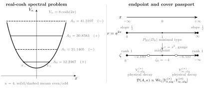
For $\kappa=4$, the left panel shows the real-cosh well, the first four parity levels, and the ground-state turning points. The right panel follows the physical contour through $r=\ee^{2x}$, whose two endpoints have Katz slope $1/2$, and then through the quadratic cover to the negative $\zeta$-ray. Both $L^2$ conditions select algebraic DCHE branches; their Abel-normalized Wronskian vanishes at an eigenvalue.

The nonlinear deformation is specifically PIII(D₈)

A fixed Heun equation and a Painlevé equation are different objects. The first is a scalar linear ODE at fixed parameters. The second governs an isomonodromic deformation of a chosen rank-two system. Their relation depends on formal type, cyclic vector, gauge, apparent-pole specialization, deformation time, monodromy chart, and boundary conditions.

For the modified-Mathieu benchmark, the minimal rank-two Lax system has slopes $(1/2,1/2)$. Its compatibility equation can be put in the standard PIII form

$$y_{TT} = \frac{y_T^2}{y} -\frac{y_T}{T} +\frac{\alpha_Py^2+\beta_P}{T} +\gamma_Py^3 +\frac{\delta_P}{y},$$

with

$$(\alpha_P,\beta_P,\gamma_P,\delta_P)=(8,-8,0,0).$$

This is the $D_8$ stratum, conventionally denoted $P_{\mathrm{III}_3}$. The comparison is

Isomonodromic type	Minimal slopes	Essential equation parameters
$P_{\mathrm{III}}(D_6)$	$(1,1)$	two
$P_{\mathrm{III}}(D_7)$	$(1/2,1)$, up to inversion	one
$P_{\mathrm{III}}(D_8)$	$(1/2,1/2)$	zero

Generic unramified DCHE geometry is associated with $D_6$. The present standard DCHE is instead a constrained quadratic pullback of the DRDCHE equation on the last row. Resolving its half-slopes does not change the underlying deformation to $D_6$.

The isomonodromic construction also separates two gates that a slogan would hide. Eliminating one component of the $D_8$ Lax system normally creates an apparent pole. On the modified-Mathieu branch, removing that pole is a tau-divisor condition

$$\mathcal T_1(\sigma,\eta,t_{\mathrm{III}})=0, \qquad \mathcal T_0(\sigma,\eta,t_{\mathrm{III}})\ne0.$$

This singularity-matching gate produces the desired scalar potential, but it does not yet impose $L^2$ decay. In a standard nonresonant monodromy chart, the endpoint connection matrix is

$$C(\sigma,\eta) = \frac1{\sin(2\pi\sigma)} \begin{pmatrix} \sin(\eta/2) &-\ii\sin(2\pi\sigma+\eta/2) \\ \ii\sin(2\pi\sigma-\eta/2) &\sin(\eta/2) \end{pmatrix}.$$

Normalizability is the independent connection gate

$$\sin\frac\eta2=0.$$

Choosing the $\eta=0$ branch and using the $D_8$ Bäcklund relation gives the exact spectral package

$$\begin{gathered} \mathcal T_0\!\left( \sigma_n+\frac12,0,t_{\mathrm{III}} \right)=0, \\ E_{\mathrm{III},n} = -t_{\mathrm{III}} \partial_{t_{\mathrm{III}}} \log\mathcal T_0(\sigma_n,0,t_{\mathrm{III}}). \end{gathered}$$

The partial derivative is taken at fixed monodromy data before the spectral root is substituted. When $\sin(2\pi\sigma)=0$, the displayed matrix chart is singular; the underlying connection problem is continued in a regular chart. A tau zero, a Heun family name, or a Painlevé label alone is therefore not a quantization condition.

Two independent solvers close the connection loop

The NumPy-only companion program uses two representations with different numerical failure modes.

1. On $x\in[0,5]$, it builds parity-reduced second-difference Jacobi matrices, locates their eigenvalues by Sturm bisection, halves the mesh, and applies second-order Richardson extrapolation.
2. On $\zeta\in(-\infty,0)$, it generates the algebraic asymptotic series recursively, launches the right-end DCHE solution, integrates it by RK4, and finds the even or odd midpoint zero. An additional two-ended run launches both algebraic bases and checks the Abel invariant at three ordinary match points.

Reproduce the calibration

From the repository root, run

python public/code/advanced-ode/modified-mathieu-dche-spectrum.py
python public/code/advanced-ode/modified-mathieu-dche-spectrum.py --mode high

The calibrated input range is $1\le\kappa\le9$ with two through eight requested levels. Optional exports are

python public/code/advanced-ode/modified-mathieu-dche-spectrum.py \
  --mode high --csv /tmp/modified-mathieu.csv
python public/code/advanced-ode/modified-mathieu-dche-spectrum.py \
  --figure-data /tmp/modified-mathieu

The CSV files contain full-precision data; the table below is rounded for reading.

For $\kappa=4$, the high-refinement profile prints

$n$	parity	real-line grid	DCHE shooting	absolute gap
0	even	12.236698387385	12.236698387584	$1.99\times10^{-10}$
1	odd	21.140503868655	21.140503869519	$8.65\times10^{-10}$
2	even	30.858318291799	30.858318292906	$1.11\times10^{-9}$
3	odd	41.310667775765	41.310667777825	$2.06\times10^{-9}$
4	even	52.440383557424	52.440383559689	$2.26\times10^{-9}$
5	odd	64.203685698682	64.203685701576	$2.90\times10^{-9}$

The last grid-to-Richardson shift is $3.43\times10^{-5}$; cancellation of the leading mesh error is why the extrapolated cross-method gaps are much smaller. The maximum DCHE refinement shift is $6.02\times10^{-9}$. At a nonspectral audit energy, the three values of the Abel-normalized Wronskian have relative spread $5.68\times10^{-13}$. These are empirical double-precision diagnostics, not rigorous error bounds. The code does not evaluate a Painlevé tau function, an NS period, or a TBA equation.

What this realization does and does not identify

Claim	Correct scope
“Modified Mathieu is Heun”	The displayed real-cosh slice becomes a DRDCHE directly and a constrained DLMF DCHE after a quadratic cover and gauge.
“The spectrum is a Wronskian zero”	Yes, for the two sectorially normalized algebraic endpoint solutions on the declared negative ray.
“DCHE means PIII(D₆)”	Only for the corresponding generic unramified formal type; this descended problem is PIII(D₈).
“A tau divisor gives the spectrum”	Only after the separate normalizability gate and the convention dictionary are imposed.
“The listed decimals are exact”	No; only the reduction and determinant characterization are exact. The decimals carry refinement diagnostics.
“This is periodic Mathieu”	No; the domain is $L^2(\mathbb R)$ and the spectrum is discrete, with no Bloch multiplier.

Common pitfalls

Importing the periodic Mathieu spectrum. The differential expression is related by a sign dictionary, but the spectral domain is different. Bloch bands and real-line $L^2$ levels answer different boundary-value problems.

Dropping the half-power gauge. The factor $s^{1/2}$ supplies both the $-1/4$ shift in $q_{\mathrm D}$ and the $1/2$ term in the even midpoint condition. Omitting it changes the equation rather than simplifying it.

Calling an irregular endpoint a Frobenius point. The displayed power series are sectorial asymptotic factors of irregular solutions. Their normalizations, Stokes sectors, and exponential competitors are part of the boundary data.

Inferring D₆ from the word “DCHE.” The direct scalar equation has half-slopes and belongs to the $D_8$ deformation. The standard DCHE appears only after a constrained quadratic cover.

Equating singularity matching with quantization. Removing the apparent pole selects the modified-Mathieu scalar equation. It does not ensure that one solution decays at both spatial ends.

Exercises

1. Translate the three passports

Starting from the mechanical operator, derive the dimensionless $(A,\kappa)$ variables and then the $(E_{\mathrm{III}},t_{\mathrm{III}})$ variables.

Solution

Set $Q=2x$, so $\partial_Q^2=\tfrac14\partial_x^2$. Multiplying

$$\left[ -\hbar_{\mathrm m}^2\partial_Q^2 +2\Lambda^2\cosh Q \right]\Psi=u\Psi$$

by $4/\hbar_{\mathrm m}^2$ gives

$$\left[ -\partial_x^2 +\frac{8\Lambda^2}{\hbar_{\mathrm m}^2}\cosh(2x) \right]\Phi = \frac{4u}{\hbar_{\mathrm m}^2}\Phi.$$

Comparison with $2\kappa\cosh(2x)$ gives $\kappa=4\Lambda^2/\hbar_{\mathrm m}^2$ and $A=4u/\hbar_{\mathrm m}^2$. Next put $Q=2x$ in the unit-kinetic PIII operator and multiply its equation by four. Then $8\sqrt{t_{\mathrm{III}}}=2\kappa$ and $4E_{\mathrm{III}}=A$, hence $t_{\mathrm{III}}=\kappa^2/16$ and $E_{\mathrm{III}}=A/4$.

2. Expose the half-slopes

Derive the DRDCHE from $r=\ee^{2x}$ and explain why both singularities have Katz slope $1/2$.

Solution

Using $\partial_x=2r\partial_r$ gives

$$\Phi_{rr}+r^{-1}\Phi_r +\left( \frac{A}{4r^2}-\frac\kappa{4r}-\frac\kappa{4r^3} \right)\Phi=0.$$

With $\Phi=r^{-1/2}\chi$, the normal-form coefficient is

$$-\frac\kappa{4r} +\frac{A+1}{4r^2} -\frac\kappa{4r^3}.$$

The pole of order three at $r=0$ produces exponential factors in $r^{-1/2}$ and therefore slope $1/2$. Invert $r$ to obtain the same order at infinity. Finally $\xi=-\kappa r/4$ yields

$$\chi_{\xi\xi} +\left[ \frac1\xi+\frac{A+1}{4\xi^2} +\frac{\kappa^2}{16\xi^3} \right]\chi=0,$$

which is the displayed DRDCHE with $q_{\mathrm{dr}}=-(A+1)/4$ and $\epsilon_{\mathrm{dr}}=\kappa^2/16$.

3. Verify the DCHE lift

Carry out the $s$, $\zeta$, and scalar-gauge substitution and recover all four DLMF parameters.

Solution

The change $s=\ee^x$ gives

$$\Phi_{ss}+s^{-1}\Phi_s +(A s^{-2}-\kappa-\kappa s^{-4})\Phi=0.$$

Write $\rho=\sqrt\kappa$ and $\Phi=s^{1/2}\ee^{-\rho(s+s^{-1})}Y$. Logarithmic differentiation gives

$$Y_{ss} +(-2\rho+2s^{-1}+2\rho s^{-2})Y_s +[-2\rho s^{-1}+(A+1/4-2\kappa)s^{-2}]Y=0.$$

Because $\zeta=-2\rho s$, divide by $(\dd\zeta/\dd s)^2=4\kappa$ and replace $s$ by $-\zeta/(2\rho)$. The coefficients become

1+\frac2\zeta-\frac{4\kappa}{\zeta^2}, \qquad \frac1\zeta-rac{2\kappa-A-1/4}{\zeta^2}.

Thus $(\alpha_{\mathrm D},\gamma_{\mathrm D},\delta_{\mathrm D},q_{\mathrm D}) =(1,2,-4\kappa,2\kappa-A-1/4)$.

4. Select the physical endpoint branches

Use the two DCHE formal bases to identify the decaying and growing Schrödinger behaviors at $s=0$ and $s=\infty$.

Solution

At $\zeta=0$, the algebraic branch is $Y\sim1$. The gauge gives $\Phi\sim s^{1/2}\ee^{-\rho/s}$, which decays. Since

$$\frac{\delta_{\mathrm D}}\zeta = \frac{-4\kappa}{-2\rho s} = \frac{2\rho}s,$$

the exponential branch instead gives $\Phi\sim s^{1/2}\ee^{+\rho/s}$ and grows. At infinity, $Y\sim\zeta^{-1}$ gives $\Phi\sim s^{-1/2}\ee^{-\rho s}$, while $Y\sim\ee^{-\zeta}\zeta^{-1}$ contributes $\ee^{2\rho s}$ and gives $\Phi\sim s^{-1/2}\ee^{+\rho s}$. Hence the algebraic branch is physical at both ends in the negative-ray chart.

5. Recover the connection and parity conditions

Prove that $\mathcal D$ is matching-point independent and derive the two midpoint residuals.

Solution

For $Y''+P(\zeta)Y'+Q(\zeta)Y=0$, Abel’s identity says $W'=-PW$. Here

$$P=1+\frac2\zeta+\frac{\delta_{\mathrm D}}{\zeta^2},$$

so

$$W(\zeta) = C\ee^{-\zeta+\delta_{\mathrm D}/\zeta}\zeta^{-2}.$$

Multiplication by $\ee^{\zeta-\delta_{\mathrm D}/\zeta}\zeta^2$ therefore leaves the constant $C$. At $x=0$, odd parity means $\Phi=0$, hence $Y(\zeta_0)=0$. For even parity differentiate $\Phi=G(s)Y(\zeta)$ with respect to $x$. Since $\dd\zeta/\dd x=\zeta$ and $\dd\log G/\dd x=1/2$ at $s=1$, the equation $\Phi'(0)=0$ becomes $\zeta_0Y'(\zeta_0)+Y(\zeta_0)/2=0$.

6. Check turning points and the deep-well constant

Find the physical turning points, prove their reciprocal pairing, and derive the $O(1)$ term in the fixed-level large-$\kappa$ spectrum.

Solution

The turning equation is $A=\kappa(s^2+s^{-2})$. Multiplication by $s^2$ gives a quadratic in $s^2$:

$$\kappa s^4-As^2+\kappa=0.$$

Its two positive roots are the displayed $s_\pm^2$ and their product is one, so $x_\pm=\log s_\pm$ are opposite. For the deep-well expansion put $x=\kappa^{-1/4}y$. Then

$$H_\kappa = 2\kappa +\sqrt\kappa(-\partial_y^2+4y^2) +\frac43y^4 +O(\kappa^{-1/2}y^6).$$

The oscillator term has eigenvalues $4n+2$. For the oscillator $-\partial_y^2+4y^2$,

$$\langle n|y^4|n\rangle = \frac{3(2n^2+2n+1)}{16}.$$

Multiplication by $4/3$ gives $(2n^2+2n+1)/4$, the required constant term.

7. Separate the two isomonodromic gates

Why is this a $D_8$ problem, and why does the apparent-pole divisor not by itself quantize the energy?

Solution

The direct DRDCHE has square-root exponential characters at both ends, so its minimal slopes are $(1/2,1/2)$. The associated PIII equation has $(\alpha_P,\beta_P,\gamma_P,\delta_P)=(8,-8,0,0)$, which is the $D_8$ stratum. The rank-one endpoints of the lifted DCHE result from resolving both half-slopes on a constrained quadratic cover; they do not create two new essential parameters and hence do not turn the deformation into $D_6$.

The condition $\mathcal T_1=0$ removes the apparent pole introduced by scalar reduction and matches the desired modified-Mathieu potential. The connection matrix can still mix recessive and dominant solutions. Setting $\sin(\eta/2)=0$ is the separate normalizability condition. Only their combination, equivalently the shifted $\mathcal T_0$ zero on the chosen branch, is spectral.

8. Audit the two numerical representations

Run the default and high profiles. What features establish that the two computations are not merely duplicate implementations?

Solution

Run

python public/code/advanced-ode/modified-mathieu-dche-spectrum.py
python public/code/advanced-ode/modified-mathieu-dche-spectrum.py --mode high

At $\kappa=4$, both profiles return alternating even and odd levels. In the high profile the first two DCHE values are

$$A_0=12.236698387584, \qquad A_1=21.140503869519,$$

and the maximum gap over six levels is $2.90\times10^{-9}$. The real-line calculation changes its coordinate mesh and uses symmetric tridiagonal Sturm counts; the DCHE calculation changes endpoint distances, asymptotic orders, and RK4 steps on a different independent variable. The Abel audit also launches from both irregular ends and remains stable across three matching points. These distinct representations expose different cutoff, discretization, and asymptotic-launch errors. Agreement is strong evidence, but the reported shifts remain empirical rather than interval-certified.

References

• NIST Digital Library of Mathematical Functions, §28.20, “Modified Mathieu Functions” and Eq. 31.12.2, the doubly confluent Heun equation. These fix the two scalar conventions used in the sign and parameter crosswalks.
• M. Bershtein, P. Gavrylenko, and A. Grassi, “Quantum Spectral Problems and Isomonodromic Deformations”, Communications in Mathematical Physics 393 (2022), 347–418, arXiv:2105.00985. Section 3 derives the modified-Mathieu $P_{\mathrm{III}_3}$ Lax specialization, connection gate, tau divisor, and exact spectrum.
• G. Bonelli, C. Iossa, D. Panea Lichtig, and A. Tanzini, “Irregular Liouville Correlators and Connection Formulae for Heun Functions”, Communications in Mathematical Physics 397 (2023), 635–727, arXiv:2201.04491. Defines the DCHE and DRDCHE normalizations and their endpoint bases.
• O. Gamayun, N. Iorgov, and O. Lisovyy, “How Instanton Combinatorics Solves Painlevé VI, V and IIIs”, Journal of Physics A 46 (2013), 335203, arXiv:1302.1832. Fixes the $P_{\mathrm{III}_3}$ parameter normalization and conformal-block tau expansions.
• M. Bershtein and A. Shchechkin, “Bäcklund Transformation of Painlevé III(D8) Tau Function”, Journal of Physics A 50 (2017), 115205, arXiv:1608.02568. Establishes the $P_{\mathrm{III}_3}=P_{\mathrm{III}}(D_8)$ tau-function framework and the Bäcklund shift used in the spectral condition.
• P. Gavrylenko and O. Lisovyy, “Pure SU(2) Gauge Theory Partition Function and Generalized Bessel Kernel”, Proceedings of Symposia in Pure Mathematics 98 (2018), 181–205, arXiv:1705.01869. Gives the Fredholm and gauge-theory realization of the $P_{\mathrm{III}}(D_8)$ tau function.
• M. van der Put and M.-H. Saito, “Moduli Spaces for Linear Differential Equations and the Painlevé Equations”, Annales de l’Institut Fourier 59 (2009), 2611–2667, arXiv:0902.1702. Classifies the formal singularity data, including the $(1/2,1/2)$ family underlying $P_{\mathrm{III}}(D_8)$.
• Y. Ohyama, H. Kawamuko, H. Sakai, and K. Okamoto, “Studies on the Painlevé Equations, V: Third Painlevé Equations of Special Type PIII(D7) and PIII(D8)”, Journal of Mathematics of the University of Tokyo 13 (2006), 145–204. Gives the $D_6\to D_7\to D_8$ coefficient strata and degeneration hierarchy.

Modified Mathieu has one hyperbolic well and no polynomial truncation mechanism. The next page keeps exponential irregular endpoints but changes the geometry to the Razavy hyperbolic double well, where special parameter values can create finite-dimensional algebraic sectors without replacing the generic exact-WKB connection problem.