Irregular States and Confluent BPZ Equations

A regular CFT puncture is labeled by a highest-weight module. When two punctures collide with their momenta held fixed, they ordinarily produce another regular insertion—or one puncture simply disappears from the outer equation. An irregular puncture appears only when positions and momenta scale together so that higher stress-tensor moments survive.

This page performs the first such collision. Two regular insertions merge at infinity into a rank-one Virasoro irregular state. A light degenerate probe then obeys an exact BPZ equation with two regular singularities and one irregular end. In the heavy–light limit, the scale derivative of an irregular classical block becomes the remaining oper coefficient, and an explicit scalar gauge gives the DLMF confluent Heun equation.

The construction in one line

$$\begin{gathered} \text{two scaled regular insertions} \longrightarrow \text{rank-one irregular state} \\ \longrightarrow \text{confluent BPZ PDE} \longrightarrow \text{rank-one oper} \longrightarrow \text{confluent Heun equation}. \end{gathered}$$

Every arrow carries normalization and scaling data. None means “set two positions equal.”

Status of the statements

Statement	Status
Virasoro constraints defining the irregular state	Exact algebraic definition
Collision formula for the chiral state	Controlled, normalization-dependent limit of analytically continued regular states
Finite-$b$ confluent BPZ equation	Exact once the irregular-state normalization and the $(2,1)$ null vector are fixed
Heavy–light reduction to an oper	Conditional on the derivative-compatible factorization hypothesis used on the preceding pages
General-Heun to confluent-Heun coefficient limit	Exact algebraic scaling, locally uniform away from the surviving singularities
Stokes or normalized connection coefficients from the scale derivative alone	Not supplied

A rank-one irregular state remembers two Virasoro moments

Place the irregular insertion at infinity and use an algebraic dual state $\langle\mathcal I_{\mu,\Lambda}|$. In the convention used on this page, it is defined by

$$\begin{aligned} \langle\mathcal I_{\mu,\Lambda}|L_0 &= \Lambda\partial_\Lambda \langle\mathcal I_{\mu,\Lambda}|, \\ \langle\mathcal I_{\mu,\Lambda}|L_{-1} &= \mu\Lambda \langle\mathcal I_{\mu,\Lambda}|, \\ \langle\mathcal I_{\mu,\Lambda}|L_{-2} &= -\frac{\Lambda^2}{4} \langle\mathcal I_{\mu,\Lambda}|, \\ \langle\mathcal I_{\mu,\Lambda}|L_{-n} &=0, \qquad n>2. \end{aligned}$$

The first line is an operator identity: $L_0$ differentiates the scale dependence of the family of states. It is not an eigenvalue equation. Likewise, $\mu$ and $\Lambda$ are irregular-state parameters, not the weight of a hidden highest-weight vector.

The distinction from an ordinary primary is structural:

State at infinity	Action of the negative modes
Dual highest-weight state $\langle\Delta	$
Rank-one irregular state $\langle\mathcal I_{\mu,\Lambda}	$

The Virasoro commutators make these conditions compatible. For example,

$$[L_{-1},L_{-2}] = L_{-3}.$$

The two prescribed eigenvalues commute, so the left-hand side vanishes on $\langle\mathcal I_{\mu,\Lambda}|$ and forces the displayed $L_{-3}$ constraint. Commutators with still lower modes propagate the vanishing conditions.

For an irregular ket at the origin, the mode indices reverse: $L_1$ and $L_2$ act diagonally and $L_n$ vanishes for $n>2$. This bra-versus-ket reversal is a convention, not a change of irregular rank.

The label “rank one” is not a substitute for these equations. Sources can rescale $(\mu,\Lambda)$, reverse signs, or use a different rank label for an $L_1$-only state. Comparisons should begin with the nonzero Virasoro modes and their eigenvalues.

The collision keeps finite first and second moments

Use the book’s centered Liouville momentum $a_{\mathrm L}$, for which

$$\Delta^{\mathrm{CFT}} = \frac{Q_{\mathrm L}^2}{4} -a_{\mathrm L}^2.$$

Introduce a collision parameter $R$ and choose

$$\begin{aligned} a_{\mathrm L,\infty}(R) &= -\frac{\mu+R}{2}, \\ a_{\mathrm L,t}(R) &= \frac{R-\mu}{2}, \\ t &= \frac{R}{\Lambda}. \end{aligned}$$

Thus $R\to\infty$ sends the moving insertion at $t$ into infinity while both conformal weights diverge. After an explicit power normalization,

$$\begin{aligned} \langle\mathcal I_{\mu,\Lambda}| \propto \lim_{R\to\infty} t^{ \Delta_t^{\mathrm{CFT}}(R) -\Delta_\infty^{\mathrm{CFT}}(R) } \langle\Delta_\infty(R)| V_{\Delta_t(R)}(t). \end{aligned}$$

The proportionality sign is intentional. An $R$-dependent but $\Lambda$-independent scalar renormalization may first be needed to make a chosen analytic normalization finite. Once it is fixed, a finite function of the remaining momenta and of $\mu$ fixes the residual three-point normalization. Neither factor changes the Virasoro constraints.

Two elementary checks expose the scaling:

$$\Delta_t^{\mathrm{CFT}}(R) -\Delta_\infty^{\mathrm{CFT}}(R) = \mu R,$$

while

$$t^{-1}R=\Lambda.$$

The divergent weights and the vanishing inverse position combine into finite first and second moments, $\mu\Lambda$ and $-\Lambda^2/4$. Those are precisely the $L_{-1}$ and $L_{-2}$ eigenvalues above. If the weights were held fixed while $t\to\infty$, both moments would vanish and the generic rank-one irregular type would not survive.

One can audit the modes before taking the limit. Put $s=\Delta_t^{\mathrm{CFT}}-\Delta_\infty^{\mathrm{CFT}}$ and denote the power-normalized state at finite $R$ by $\langle I_R|$. The primary commutator gives, for $k\geq1$,

$$\begin{aligned} \langle I_R|L_{-k} = -t^{-k} \left[ t\partial_t +(1-k)\Delta_t^{\mathrm{CFT}} -s \right] \langle I_R|. \end{aligned}$$

At fixed $R$, $t\partial_t=-\Lambda\partial_\Lambda$. The derivative term is suppressed by $t^{-k}$, while the divergent part of $\Delta_t^{\mathrm{CFT}}$ survives only for $k\leq2$. Substitution gives $\mu\Lambda$, $-\Lambda^2/4$, and zero for $k>2$, respectively.

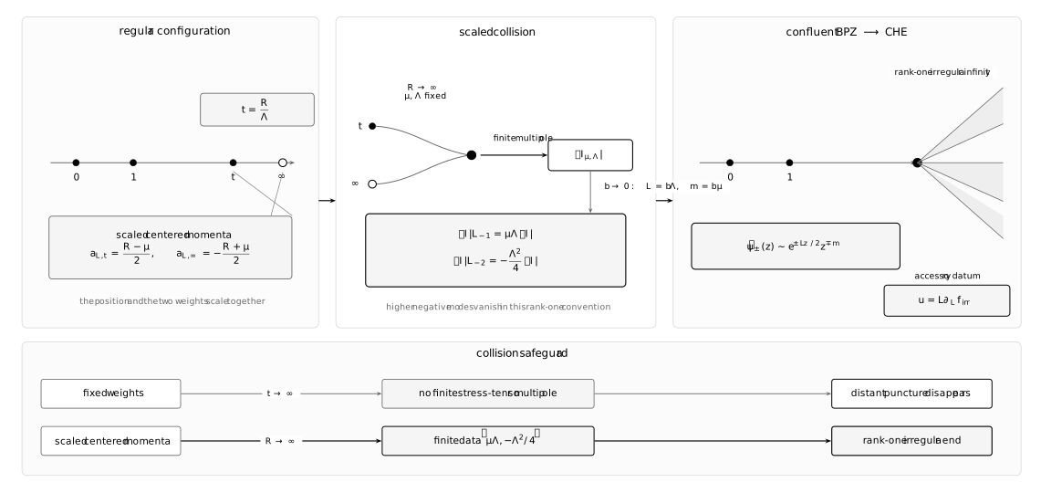
A collision is a correlated limit of position and momenta. Fixed weights make the distant puncture disappear; scaled centered momenta retain the finite Virasoro moments $\mu\Lambda$ and $-\Lambda^2/4$, which become the formal data of the rank-one irregular end.

This construction is an analytic chiral limit. The intermediate regular weights need not lie in a unitary spectrum, and a full Liouville correlator requires additional structure constants, antiholomorphic data, and a contour prescription.

The exact confluent BPZ equation is still a PDE

Throughout this finite-$b$ subsection, $\Delta_j$ abbreviates $\Delta_j^{\mathrm{CFT}}$; in particular, $\Delta_{2,1}$ is the weight of the $(2,1)$ degenerate field.

Insert the book’s light degenerate field $V_{-b/2}(z)$ between a regular state at zero, a regular primary at one, and the irregular bra:

$$\mathcal G(z,\Lambda) := \left\langle \mathcal I_{\mu,\Lambda} \right| V_1(1) V_{-b/2}(z) \left| \Delta_0 \right\rangle.$$

The null relation and the irregular Ward identities give

$$\begin{aligned} 0 ={}& \left[ b^{-2}\partial_z^2 - \left( \frac1z+\frac1{z-1} \right)\partial_z \right. \\ &\left. + \frac{ \Lambda\partial_\Lambda -\Delta_{2,1} -\Delta_1 -\Delta_0 }{ z(z-1) } \right. \\ &\left. + \frac{\Delta_1}{(z-1)^2} + \frac{\Delta_0}{z^2} + \frac{\mu\Lambda}{z} - \frac{\Lambda^2}{4} \right] \mathcal G. \end{aligned}$$

This is the confluent analogue of the five-insertion BPZ equation. The regular modulus has been replaced by the irregular scale $\Lambda$, but its derivative has not disappeared. At finite $b$ the equation is a PDE in $(z,\Lambda)$.

The singularity structure is already visible:

Point	Exact BPZ behavior
$z=0$	Regular singularity controlled by $\Delta_0$
$z=1$	Regular singularity controlled by $\Delta_1$
$z=\infty$	Irregular terms $\mu\Lambda/z-\Lambda^2/4$

If the insertion at one is omitted, the same Ward calculation gives the one-regular-point equation

$$\left[ b^{-2}\partial_z^2 -\frac1z\partial_z +\frac{\Delta_0}{z^2} +\frac{\mu\Lambda}{z} -\frac{\Lambda^2}{4} \right]\mathcal G_{\mathrm W} =0.$$

After a scalar power gauge this is Whittaker’s equation. It is the rigid confluent-hypergeometric benchmark behind the nonrigid confluent-Heun problem.

More explicitly, set

$$\Delta_0^{\mathrm{CFT}} = \frac{Q_{\mathrm L}^2}{4} -a_{\mathrm L,0}^2, \qquad x=b\Lambda z, \qquad \mathcal G_{\mathrm W} = z^{b^2/2}w(x).$$

Then

$$\frac{\dd^2w}{\dd x^2} + \left[ -\frac14 +\frac{b\mu}{x} +\frac{ \frac14-b^2a_{\mathrm L,0}^2 }{x^2} \right]w =0.$$

The two regular-end branches are proportional to

$$z^{b^2/2} M_{b\mu,\,\pm b a_{\mathrm L,0}} (b\Lambda z).$$

Whittaker $W$-type solutions instead encode sectorial asymptotics at the irregular end. Their connection coefficients are not needed for the confluent-Heun derivation below.

Nearby irregular patterns are different problems

Virasoro insertion pattern	ODE benchmark after null decoupling
Rank one at infinity, no regular insertion at one	Whittaker / confluent hypergeometric
Rank one at infinity plus regular insertions at zero and one	Confluent BPZ; confluent Heun after the classical limit
An $L_1$-only state, called rank one-half in the main source	Bessel or reduced confluent-Heun limits
Rank-one states at both ends	Doubly confluent BPZ / doubly confluent Heun

The Heun confluence hierarchy keeps these collision patterns separate. This page derives only the second row.

Heavy–light factorization produces the irregular oper

Take $b\to0$ in a fixed complex sector and scale

$$\begin{aligned} b\,a_{\mathrm L,0} &\longrightarrow \frac{\theta_0}{2}, & b\,a_{\mathrm L,1} &\longrightarrow \frac{\theta_1}{2}, \\ b\mu&\longrightarrow m, & b\Lambda&\longrightarrow L. \end{aligned}$$

Then

$$\delta_i := \lim_{b\to0}b^2\Delta_i^{\mathrm{CFT}} = \frac{1-\theta_i^2}{4}, \qquad i\in\{0,1\}.$$

Fix a heavy internal channel as well:

$$b^2\Delta_{\mathrm{int}}^{\mathrm{CFT}} \longrightarrow \delta_{\mathrm{int}} = \frac{1-\theta_{\mathrm{int}}^2}{4}.$$

Let $\mathcal B_{\mathrm{irr}}(\Lambda)$ be the background irregular block obtained by removing the degenerate probe. Define its classical scale coordinate directly by

$$u(L) := \lim_{b\to0} b^2\Lambda\partial_\Lambda \Log\mathcal B_{\mathrm{irr}}(\Lambda) \bigg|_{\Lambda=L/b}.$$

This derivative definition is safer than taking $\lim b^2\Log\mathcal B_{\mathrm{irr}}(L/b)$ directly: the leading power can leave an $L$-independent term proportional to $\Log b$. After choosing an $L$-independent subtraction, introduce a primitive $f_{\mathrm{irr}}$ by

$$u(L) = L\partial_Lf_{\mathrm{irr}}(L).$$

Now factor

$$\mathcal G(z,\Lambda) = \mathcal B_{\mathrm{irr}}(\Lambda) \Psi_b(z;L).$$

Assume that $\Psi_b$ and its first two $z$-derivatives converge locally uniformly to $\psi$, and that

$$b^2\Lambda\partial_\Lambda\Psi_b \longrightarrow 0$$

locally uniformly on the same domain. This is the derivative-compatible irregular heavy–light hypothesis.

After multiplying the exact BPZ equation by $b^2$, every surviving term has a transparent origin:

Finite-$b$ quantity	Classical limit
$b^2\Delta_i^{\mathrm{CFT}}$	$\delta_i$
$b^2\Lambda\partial_\Lambda\Log\mathcal B_{\mathrm{irr}}$	$u$
$b^2\mu\Lambda$	$mL$
$b^2\Lambda^2$	$L^2$
$b^2\Delta_{2,1}$ and the first-derivative term	$0$

The limiting probe equation is

$$\left[ \partial_z^2 +T_{\mathrm{irr}}(z;L) \right]\psi(z;L) =0,$$

with

$$\begin{aligned} T_{\mathrm{irr}}(z;L) ={}& \frac{\delta_0}{z^2} + \frac{\delta_1}{(z-1)^2} \\ &+ \frac{ u-\delta_0-\delta_1 }{ z(z-1) } + \frac{mL}{z} - \frac{L^2}{4}. \end{aligned}$$

This is the rank-one irregular counterpart of the four-pole oper on the preceding page. The single coefficient $u$ is supplied by a scale derivative rather than a position derivative.

The leading irregular power must be retained

Suppose the full and unit-leading irregular blocks are related by

$$\mathcal B_{\mathrm{irr}}(\Lambda) = \Lambda^{\Delta_{\mathrm{int}}} \widehat{\mathcal B}_{\mathrm{irr}}(\Lambda).$$

After absorbing an $L$-independent normalization into the chosen branch,

$$f_{\mathrm{irr}}(L) = \delta_{\mathrm{int}}\Log L +\widehat f_{\mathrm{irr}}(L),$$

and therefore

$$u(L) = \delta_{\mathrm{int}} +L\partial_L\widehat f_{\mathrm{irr}}(L).$$

For a unit-leading small-$L$ series,

$$u(L) = \delta_{\mathrm{int}} +O(L).$$

At $L=0$ the irregular terms vanish and the oper reduces to the three-regular-point coefficient

$$\begin{aligned} T_0(z) ={}& \frac{\delta_0}{z^2} + \frac{\delta_1}{(z-1)^2} \\ &+ \frac{ \delta_{\mathrm{int}} -\delta_0 -\delta_1 }{ z(z-1) }. \end{aligned}$$

Thus the collision family returns to its hypergeometric boundary with the chosen internal exponent at infinity. Dropping the leading irregular power would fail this check.

Pole order and formal exponentials identify rank one

For large $z$, the normal-form coefficient has the expansion

$$T_{\mathrm{irr}}(z;L) = -\frac{L^2}{4} +\frac{mL}{z} +\frac{u}{z^2} +O(z^{-3}).$$

Under inversion $w=1/z$, the projective connection transforms as

$$\widetilde T(w) = w^{-4}T_{\mathrm{irr}}(1/w),$$

because inversion is Möbius and its Schwarzian vanishes. Hence

$$\widetilde T(w) = -\frac{L^2}{4w^4} +\frac{mL}{w^3} +\frac{u}{w^2} +O(w^{-1}).$$

For $L\neq0$, the fourth-order pole is the scalar normal-form signature of an unramified rank-one irregular singularity.

The two formal branches begin as

$$\widehat\psi_\pm(z) = \exp\left( \pm\frac{Lz}{2} \right) z^{\mp m} \left[ 1+O(z^{-1}) \right].$$

The exponent difference is $Lz$. Its real part changes sign on $\operatorname{Re}(Lz)=0$, so different sectors have different dominant branches. Actual analytic solutions asymptotic to $\widehat\psi_\pm$ are sectorial and are related across sector boundaries by Stokes matrices. The parameter $m$ is formal monodromy data; it is not a pair of ordinary Frobenius exponents at infinity.

The DLMF confluent-Heun dictionary is exact

Use the DLMF confluent Heun equation

$$\begin{aligned} y'' &+ \left( \frac{\gamma_{\mathrm C}}z + \frac{\delta_{\mathrm C}}{z-1} + \epsilon_{\mathrm C} \right)y' \\ &+ \frac{ \alpha_{\mathrm C}z-q_{\mathrm C} }{ z(z-1) }y =0. \end{aligned}$$

The subscript $\mathrm C$ keeps these canonical parameters distinct from CFT weights and centered momenta. On a simply connected patch, set

$$\begin{aligned} y(z) ={}& \exp\left( -\frac{\epsilon_{\mathrm C}z}{2} \right) z^{-\gamma_{\mathrm C}/2} (1-z)^{-\delta_{\mathrm C}/2} \psi(z). \end{aligned}$$

The exact inverse dictionary from the irregular oper is

$$\begin{aligned} \gamma_{\mathrm C} &= 1-\theta_0, & \delta_{\mathrm C} &= 1-\theta_1, \\ \epsilon_{\mathrm C} &= L, & \alpha_{\mathrm C} &= L \left( m+\frac{\gamma_{\mathrm C}+\delta_{\mathrm C}}2 \right), \end{aligned}$$

together with

$$\begin{aligned} q_{\mathrm C} ={}& \frac14 - \frac{ \left( \gamma_{\mathrm C}+\delta_{\mathrm C}-1 \right)^2 }{4} \\ &+ L \left( m+\frac{\gamma_{\mathrm C}}2 \right) -u. \end{aligned}$$

Equivalently, the forward accessory map is

$$\begin{aligned} u ={}& \frac14 -q_{\mathrm C} +\alpha_{\mathrm C} \\ &- \frac{ \left( \gamma_{\mathrm C}+\delta_{\mathrm C}-1 \right)^2 }{4} - \frac{ \delta_{\mathrm C}\epsilon_{\mathrm C} }{2}. \end{aligned}$$

The regular standard-form exponents are

$$\begin{array}{c|c} z=0 & 0,\ 1-\gamma_{\mathrm C}=\theta_0 \\ z=1 & 0,\ 1-\delta_{\mathrm C}=\theta_1 \end{array}.$$

For $L=\epsilon_{\mathrm C}\neq0$, the two standard-form asymptotic branches at infinity are instead

$$\begin{aligned} y_+(z) &\sim z^{-\alpha_{\mathrm C}/\epsilon_{\mathrm C}}, \\ y_-(z) &\sim \exp(-\epsilon_{\mathrm C}z) z^{ \alpha_{\mathrm C}/\epsilon_{\mathrm C} -\gamma_{\mathrm C} -\delta_{\mathrm C} }. \end{aligned}$$

Dividing by the scalar gauge recovers $\widehat\psi_\pm$. This simultaneously checks the exponential signs and the definition of $m$. At $L=0$, the dictionary also has $\alpha_{\mathrm C}=0$: the equation lies on its hypergeometric boundary, and $m$ is no longer an independent differential-equation parameter.

The ODE confluence mirrors the CFT collision

The coefficient limit can be checked independently of CFT. Let the fourth regular singularity of the general Heun equation be $A\to\infty$ and fix target confluent parameters with $\epsilon_{\mathrm C}\neq0$. Scale

$$\begin{aligned} \epsilon_{\mathrm G} &= -A\epsilon_{\mathrm C}, \\ \alpha_{\mathrm G} &= \frac{\alpha_{\mathrm C}}{\epsilon_{\mathrm C}}, \\ \beta_{\mathrm G} &= -A\epsilon_{\mathrm C} +\gamma_{\mathrm C} +\delta_{\mathrm C} -1 -\frac{\alpha_{\mathrm C}}{\epsilon_{\mathrm C}}, \\ q_{\mathrm G} &= -Aq_{\mathrm C}. \end{aligned}$$

The general-Heun Fuchs relation holds exactly. For fixed $z$ away from $0$ and $1$,

$$\frac{\epsilon_{\mathrm G}}{z-A} \longrightarrow \epsilon_{\mathrm C},$$

and

$$\frac{ \alpha_{\mathrm G}\beta_{\mathrm G}z-q_{\mathrm G} }{ z(z-1)(z-A) } \longrightarrow \frac{ \alpha_{\mathrm C}z-q_{\mathrm C} }{ z(z-1) }.$$

This is the same mechanism as the CFT collision: a point moves to infinity while selected parameters diverge so that finite first and second moments remain. The Heun confluence page proves local-uniform coefficient and initial-value solution convergence and records the $O(A^{-1})$ remainder.

The matching concerns the equation and fixed-base-point solutions on an outer domain. Frobenius bases attached to the moving singularity generally need singular normalization before they approach sectorial bases of the irregular equation.

The regular accessory has a finite irregular remainder

The same collision can be checked directly in normal form. Start from the four-pole oper

$$\begin{aligned} T_A(z) ={}& \frac{\delta_0}{z^2} +\frac{\delta_1}{(z-1)^2} +\frac{\delta_A}{(z-A)^2} \\ &+ \frac{\Xi_A}{z(z-1)} + \frac{ A(A-1)c_A }{ z(z-1)(z-A) }, \end{aligned}$$

where

$$\Xi_A = \delta_\infty-\delta_0-\delta_A-\delta_1.$$

Choose exponent representatives and the accessory scaling

$$\begin{aligned} \theta_A&=AL-m, & \theta_\infty&=-AL-m, \\ c_A&=-mL-\frac{u}{A}+O(A^{-2}), & \delta_\nu&=\frac{1-\theta_\nu^2}{4}. \end{aligned}$$

Then $\Xi_A=-ALm-\delta_0-\delta_1$, and direct expansion gives $T_A\to T_{\mathrm{irr}}$ locally uniformly away from $0$ and $1$. In this normalization the irregular energy is the finite remainder

$$u = -\lim_{A\to\infty} A\left(c_A+mL\right).$$

Thus the regular accessory itself tends to $-mL$; subtracting that collision term and rescaling extracts the classical irregular-block coordinate. Here $c_A=(\partial_A f_{\mathrm{reg}})_{\{\delta_\nu\}}$ is defined with the regular weights held fixed. Differentiating along the collision path without accounting for their variation gives a different—and incorrect—remainder.

What changes when a regular point becomes irregular

The collision changes the correct local data, not merely the function name.

Regular point before collision	Rank-one irregular point after collision
Two Frobenius powers	Two formal exponential-power branches
One local monodromy matrix	Formal monodromy plus Stokes matrices
Punctured disk	Overlapping sectors
Resonance from an integer exponent difference	Formal resonance and Stokes degeneracies, analyzed separately
Frobenius-normalized connection matrix	Sectorially normalized connection or Stokes matrix

The classical irregular block supplies $u$, hence the differential equation. It does not by itself specify sector labels, summation directions, asymptotic normalizations, Stokes multipliers, or a regular-to- irregular connection matrix. Chapter 7 adds the irregular fusion factors and normalization data needed for those connection problems.

Common pitfalls

Sending a puncture away with fixed weights. Then its polar moments vanish on the outer domain. The generic confluent equation requires a compensating momentum and accessory scaling.

Calling the irregular state a highest-weight state. Its $L_0$ action is a scale derivative, and two higher moments act diagonally. It belongs to a Whittaker-type Virasoro module rather than an ordinary Verma module.

Treating the exact confluent BPZ equation as an ODE. The term $\Lambda\partial_\Lambda$ survives at finite $b$. It becomes the number $u$ only after a derivative-compatible classical factorization.

Using a unit-leading block without restoring its power. The full scale derivative contains $\delta_{\mathrm{int}}$. Omitting it gives the wrong $L\to0$ hypergeometric boundary.

Writing $q_{\mathrm C}=u$. The irregular block derivative is the normal-form coordinate $u$. The standard confluent-Heun accessory $q_{\mathrm C}$ differs by the displayed scalar-gauge shift.

Assigning Frobenius exponents to the irregular end. Infinity has formal exponential powers and Stokes sectors for $L\neq0$. The regular limit $L=0$ is a different singularity stratum.

Exercises

1. Check the irregular Virasoro constraints

Use the Virasoro commutator to show that the prescribed $L_{-1}$ and $L_{-2}$ eigenvalues imply $\langle\mathcal I_{\mu,\Lambda}|L_{-3}=0$.

Solution

Since

$$[L_{-1},L_{-2}] = L_{-3},$$

the left-hand side acts by

$$(\mu\Lambda) \left( -\frac{\Lambda^2}{4} \right) - \left( -\frac{\Lambda^2}{4} \right) (\mu\Lambda) =0.$$

Therefore the action of $L_{-3}$ vanishes. Commuting $L_{-1}$ with $L_{-n}$ then propagates the higher vanishing constraints.

2. Audit the collision normalization

Starting from the two centered momenta, compute $\Delta_t^{\mathrm{CFT}}-\Delta_\infty^{\mathrm{CFT}}$.

Solution

The common $Q_{\mathrm L}^2/4$ cancels, so

$$\begin{aligned} \Delta_t^{\mathrm{CFT}} -\Delta_\infty^{\mathrm{CFT}} &= -\frac{(\mu-R)^2}{4} +\frac{(\mu+R)^2}{4} \\ &= \mu R. \end{aligned}$$

Thus the normalizing power is $t^{\mu R}$. Together with $t=R/\Lambda$, it removes the divergent dilation weight while leaving finite $\Lambda$-dependent Virasoro moments.

3. Recover the classical oper term by term

Multiply the exact BPZ equation by $b^2$, insert the heavy–light factorization, and recover $T_{\mathrm{irr}}$.

Solution

The background logarithmic derivative gives

$$b^2\Lambda\partial_\Lambda \Log\mathcal B_{\mathrm{irr}} \longrightarrow u.$$

The heavy weights give $\delta_0$ and $\delta_1$, while

$$b^2\mu\Lambda\to mL, \qquad b^2\Lambda^2\to L^2.$$

The light degenerate weight and the first-derivative term are multiplied by $b^2$ and vanish. The coefficient of $1/[z(z-1)]$ is therefore $u-\delta_0-\delta_1$, giving exactly the displayed oper.

4. Verify the rank at infinity

Invert $z=1/w$ and derive both the pole order and the leading formal branches.

Solution

The half-density transformation gives

$$\widetilde T(w) = w^{-4}T(1/w) = -\frac{L^2}{4w^4} +\frac{mL}{w^3} +O(w^{-2}).$$

For $L\neq0$, this is an unramified rank-one irregular singularity in scalar normal form. For a formal ansatz

$$\psi = \exp\left( \frac{sLz}{2} \right)z^\rho \left[ 1+O(z^{-1}) \right], \qquad s=\pm1,$$

the constant terms cancel and the $z^{-1}$ coefficient is $L(s\rho+m)$. Hence $\rho=-sm$, which gives $\widehat\psi_\pm$.

5. Derive the scale-normalization shift

Assume $\mathcal B_{\mathrm{irr}} =\Lambda^{\Delta_{\mathrm{int}}} \widehat{\mathcal B}_{\mathrm{irr}}$. Find $u$ in terms of the unit-leading classical block.

Solution

Taking the logarithm, multiplying by $b^2$, and holding $L=b\Lambda$ fixed in the classical scaling gives

$$f_{\mathrm{irr}} = \delta_{\mathrm{int}}\Log L +\widehat f_{\mathrm{irr}}$$

up to an $L$-independent term. Therefore

$$u = L\partial_Lf_{\mathrm{irr}} = \delta_{\mathrm{int}} +L\partial_L\widehat f_{\mathrm{irr}}.$$

6. Check the confluent-Heun accessory map

Apply the scalar gauge to the DLMF equation and recover the displayed formula for $u$.

Solution

For

$$p(z) = \frac{\gamma_{\mathrm C}}z +\frac{\delta_{\mathrm C}}{z-1} +\epsilon_{\mathrm C},$$

the normal coefficient is

$$T = \frac{\alpha_{\mathrm C}z-q_{\mathrm C}}{z(z-1)} -\frac12p' -\frac14p^2.$$

Its double-pole coefficients are $\gamma_{\mathrm C}(2-\gamma_{\mathrm C})/4$ and $\delta_{\mathrm C}(2-\delta_{\mathrm C})/4$. Matching the constant and the sum of its simple-pole residues gives

$$L=\epsilon_{\mathrm C}, \qquad m = \frac{\alpha_{\mathrm C}}{\epsilon_{\mathrm C}} -\frac{\gamma_{\mathrm C}+\delta_{\mathrm C}}2.$$

Matching the remaining $1/[z(z-1)]$ coefficient gives

$$\begin{aligned} u ={}& \frac14-q_{\mathrm C}+\alpha_{\mathrm C} \\ &- \frac{ (\gamma_{\mathrm C}+\delta_{\mathrm C}-1)^2 }{4} - \frac{\delta_{\mathrm C}\epsilon_{\mathrm C}}2. \end{aligned}$$

7. Show why an unscaled moving pole is insufficient

Let $A\to\infty$ in the general Heun equation while every canonical parameter stays bounded. Determine the outer coefficient limit.

Solution

For fixed $z$,

$$\frac{\epsilon_{\mathrm G}}{z-A} = O(A^{-1}),$$

and

$$\frac{ \alpha_{\mathrm G}\beta_{\mathrm G}z-q_{\mathrm G} }{ z(z-1)(z-A) } = O(A^{-1}).$$

The limiting equation is

$$y'' + \left( \frac{\gamma_{\mathrm G}}z + \frac{\delta_{\mathrm G}}{z-1} \right)y' =0,$$

a degenerate Fuchsian equation. The generic confluent-Heun terms survive only under the divergent parameter scaling used on this page.

References

• D. Gaiotto, “Asymptotically Free $\mathcal N=2$ Theories and Irregular Conformal Blocks”, 2009. Introduces the Whittaker-type Virasoro states that encode asymptotically free conformal blocks.
• D. Gaiotto and J. Teschner, “Irregular Singularities in Liouville Theory and Argyres–Douglas Type Gauge Theories, I”, Journal of High Energy Physics 2012 (2012), 50. Develops irregular modules, collision limits, block bases, and their normalization data.
• G. Bonelli, C. Iossa, D. Panea Lichtig, and A. Tanzini, “Irregular Liouville Correlators and Connection Formulae for Heun Functions”, Communications in Mathematical Physics 397 (2023), 635–727. Gives the rank-one collision, exact confluent BPZ equation, semiclassical oper, and normalization-aware confluent-Heun dictionary used here.
• NIST Digital Library of Mathematical Functions, §31.12 and equation 31.12.1, for the canonical confluent Heun equation and its two regular singularities plus rank-one irregular singularity at infinity.
• NIST Digital Library of Mathematical Functions, §13.14, for Whittaker’s equation, canonical solutions, and the rigid confluent-hypergeometric benchmark.
• J. Lenells and J. Roussillon, “Confluent Conformal Blocks of the Second Kind”, Journal of High Energy Physics 2020 (2020), 133. Constructs conformal-block bases adapted to sectorial asymptotics at an irregular singularity and relates their degenerate limits to confluent BPZ solutions.